Machine & Reinforcement Learning in SUMO Traffic Simulator

Tutorial objective

From traffic simulation to intelligent control

The tutorial develops two reinforcement-learning traffic signal controllers — Q-learning and Deep Q-learning — and compares them with a static/fixed-timing traffic signal. The study intersection is intentionally a random tutorial intersection, not a calibrated real-world site.

Controller 1

Fixed timing — Traci5.py

Controller 2 & 3

Q-learning — Traci6.py
Deep Q-learning — Traci7.py

1 • Fundamentals

Where reinforcement learning fits in machine learning

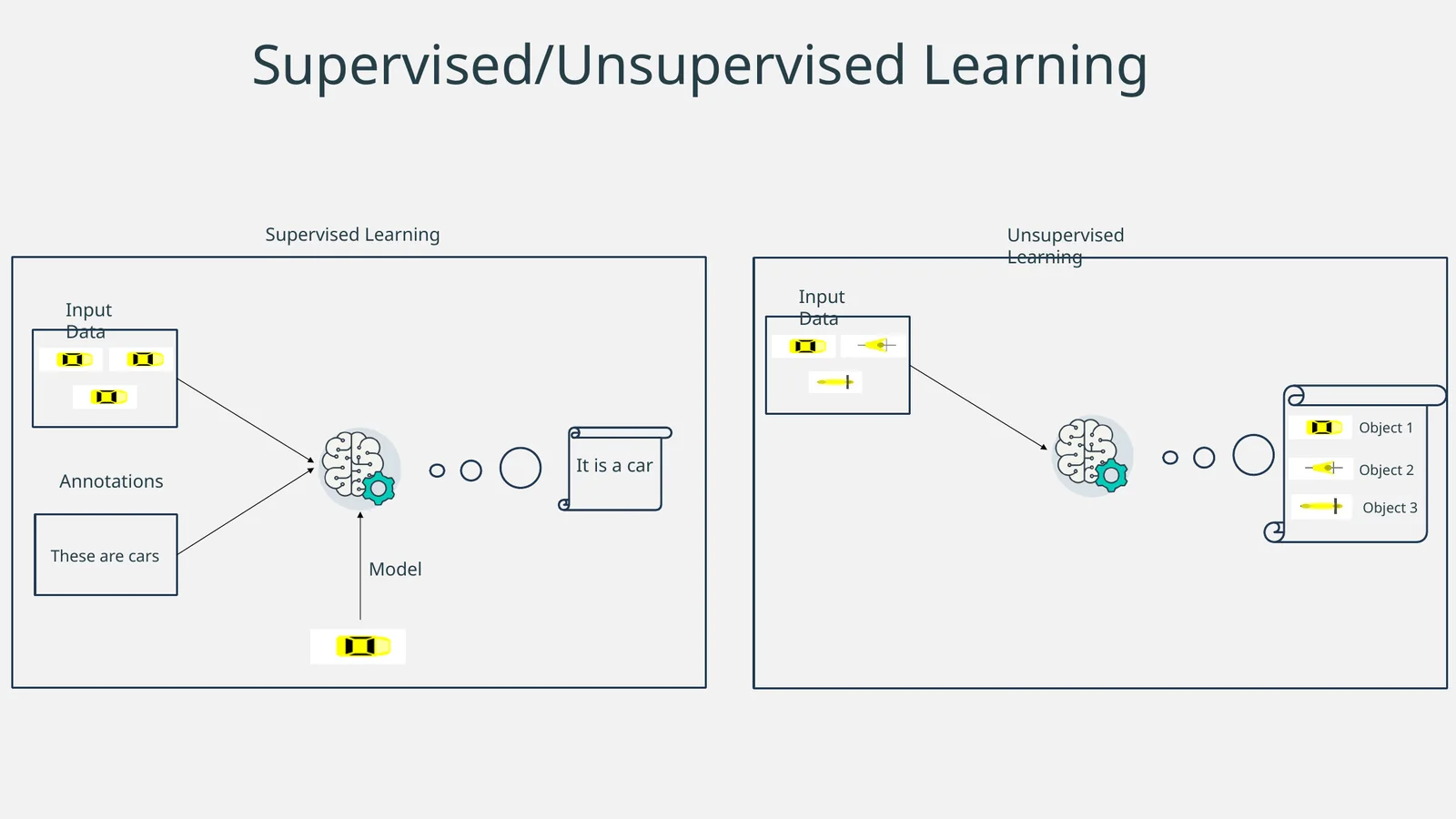
The deck first separates supervised, unsupervised, semi-supervised, and reinforcement learning. Supervised learning uses annotated examples; unsupervised learning seeks patterns without those labels. Reinforcement learning instead learns from interaction with an environment.

Supervised and unsupervised learning illustration — Supervised vs. unsupervised learning from the RoadwayVR tutorial.

SupervisedUnsupervisedSemi-supervisedReinforcement learning

2 • Reinforcement learning

The traffic signal becomes an RL agent

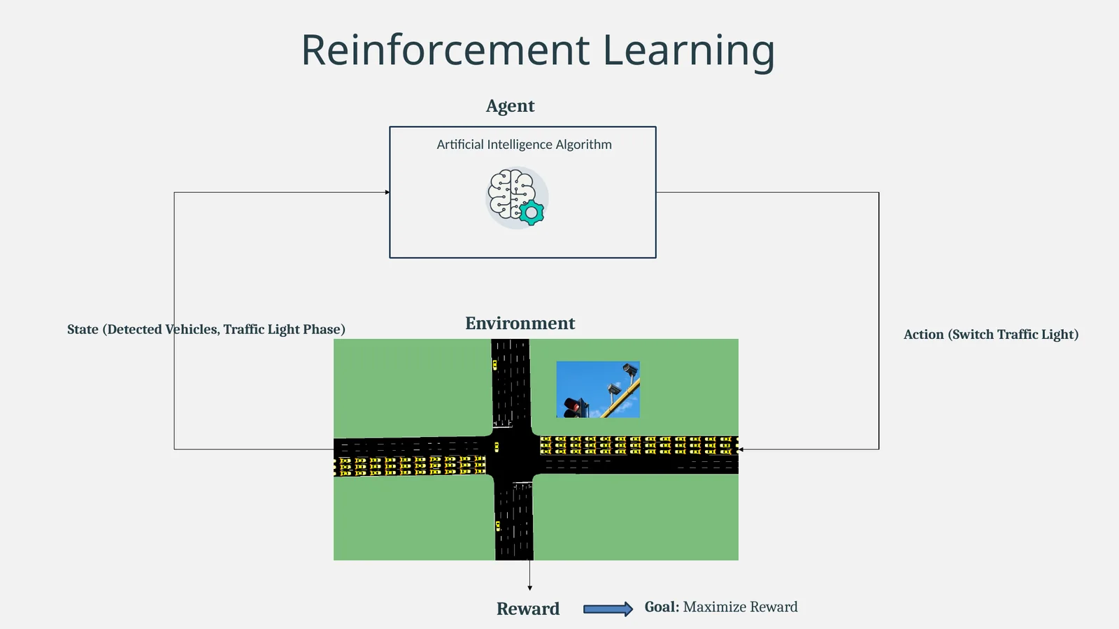
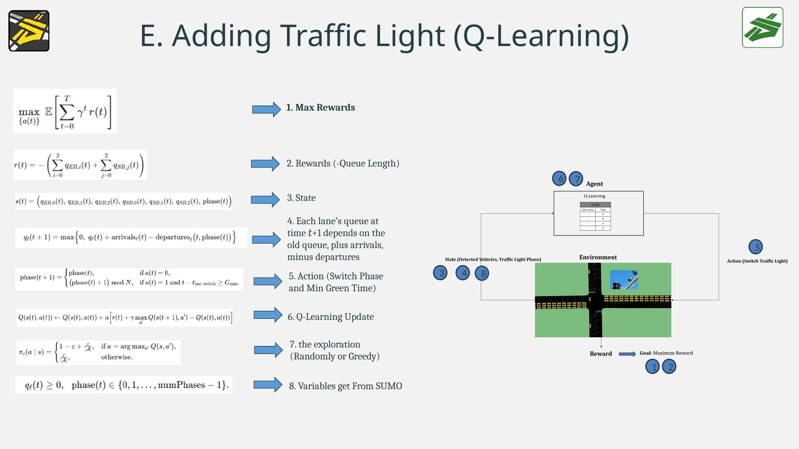
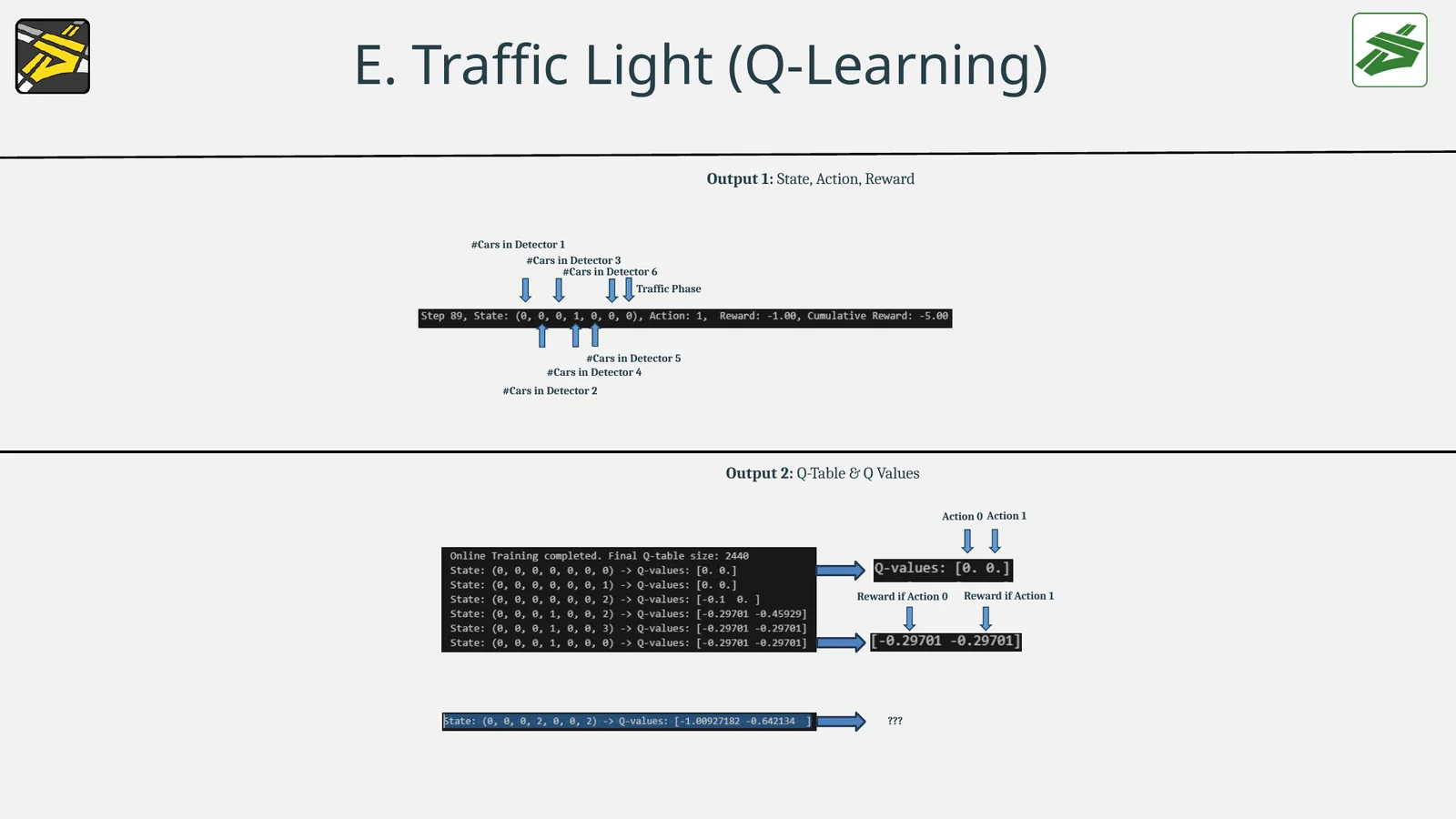
For the traffic-signal problem, the tutorial defines the state from detected vehicles and the traffic-light phase, the action as keeping or switching the traffic light, and the reward so the agent learns to maximize long-term performance.

Statedetector queues + signal phase

AgentQ-learning / DQN

Actionkeep or switch phase

EnvironmentSUMO intersection

Rewardbased on queue length

Reinforcement learning loop for a SUMO traffic signal — State → agent → action → SUMO environment → reward.

3 • State design

Collect the state from SUMO detectors

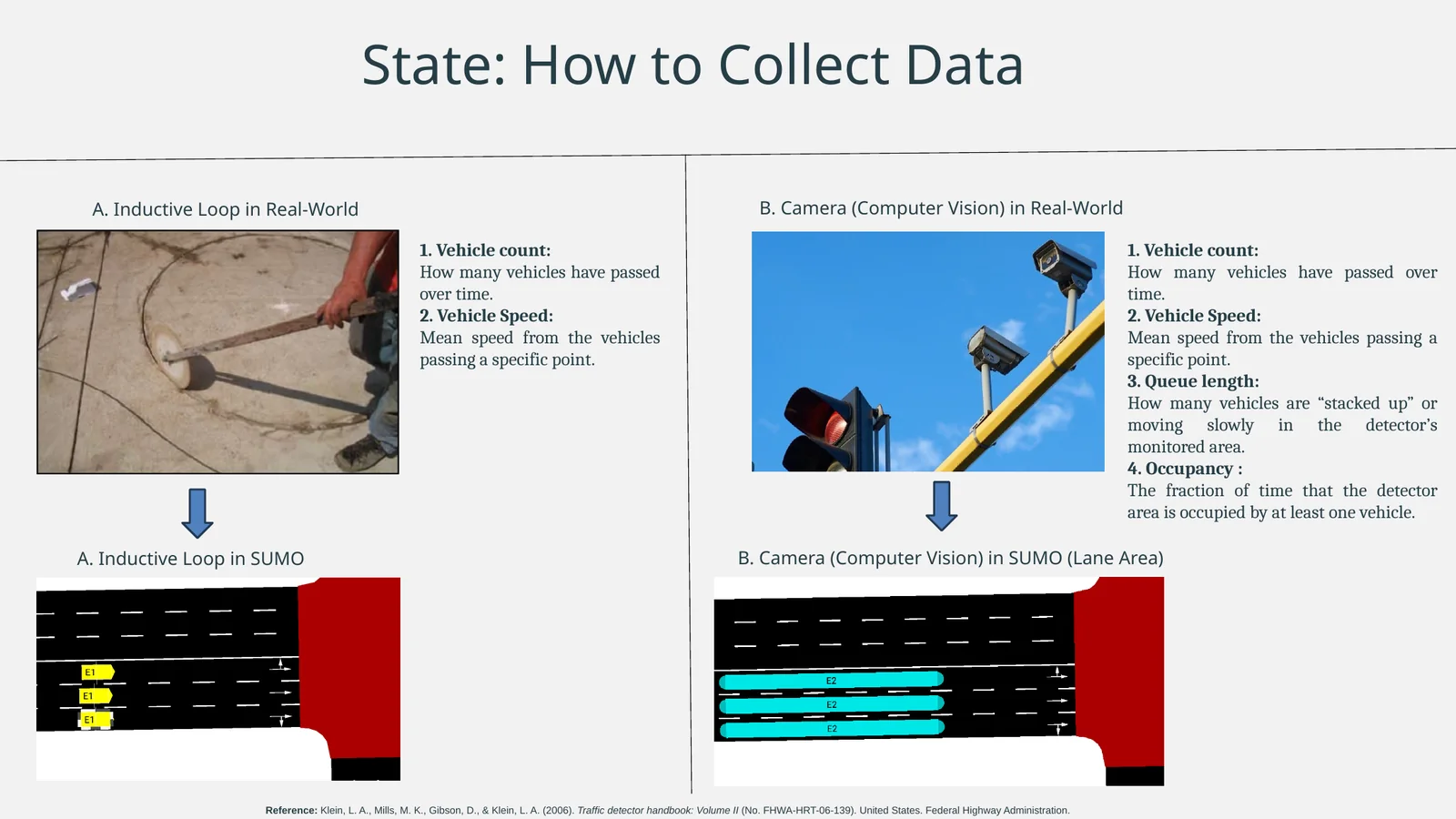
The tutorial connects real-world detection concepts to SUMO: inductive loops correspond to point detection, while SUMO lane-area detectors represent a camera-like monitored road segment.

Inductive-loop style data

Vehicle count and mean vehicle speed at a specific point.

Lane-area / camera-style data

Vehicle count, mean speed, queue length, and occupancy over a monitored area.

Real-world and SUMO detector comparison — Real-world detectors and their SUMO counterparts.

Detector variables used by the RL controller: six lane queues plus the current traffic-signal phase.

s(t) = (q_EB,0, q_EB,1, q_EB,2, q_SB,0, q_SB,1, q_SB,2, phase(t))

4 • Tutorial study

A small intersection for a controlled comparison

The workflow follows the traffic-microsimulation process: analysis planning, data collection, base model development, error checking, calibration, and alternatives analysis. For this tutorial, error checking and calibration are noted but skipped because the example does not use real-world calibration data.

Goal

Develop Q-learning and Deep Q-learning traffic-signal control.

Benchmark

Compare both RL controllers with a static/fixed-timing signal.

Tutorial scope: traffic volume, speed, car-following, lane-changing, and vehicle-type parameters use default SUMO values in the deck.

5 • SUMO implementation

Build the base model before adding intelligence

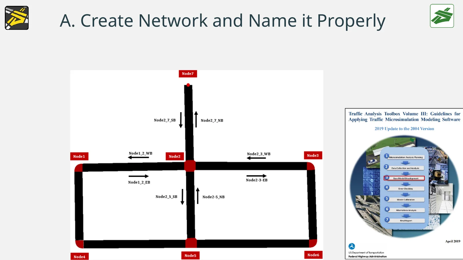
Create and name the network

Create the tutorial intersection and give the network elements consistent names so TraCI and detector logic can reference them reliably.

Tutorial SUMO intersection and named network — The tutorial intersection used for the ML/RL example.

Add traffic demand and vehicle types

The deck shows example flows F_0, F_1, and F_2 with values of 1800, while vehicle types remain at SUMO defaults.

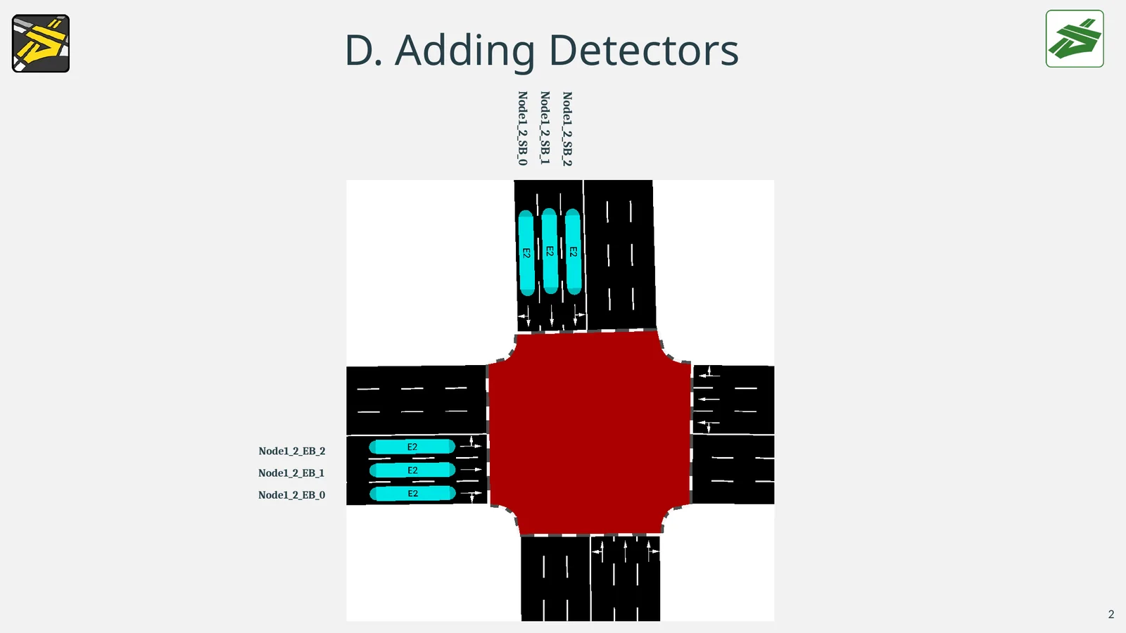
Add six lane-area detectors

The detector IDs shown in the tutorial are Node1_2_EB_0, Node1_2_EB_1, Node1_2_EB_2, Node1_2_SB_0, Node1_2_SB_1, and Node1_2_SB_2.

Six lane area detectors around the tutorial intersection — Six SUMO lane-area detectors form the traffic-state inputs.

Prepare the three signal-control scripts

Fixed timing uses Traci5.py, Q-learning uses Traci6.py, and Deep Q-learning uses Traci7.py.

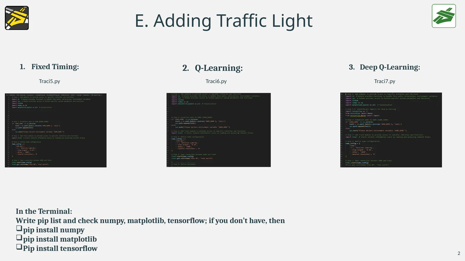
Fixed timing, Q-learning and Deep Q-learning Python scripts — The three controller implementations shown in the tutorial.

Check the Python packages

pip list
pip install numpy
pip install matplotlib
pip install tensorflow

6 • Q-learning

Learn a signal-control policy with a Q-table

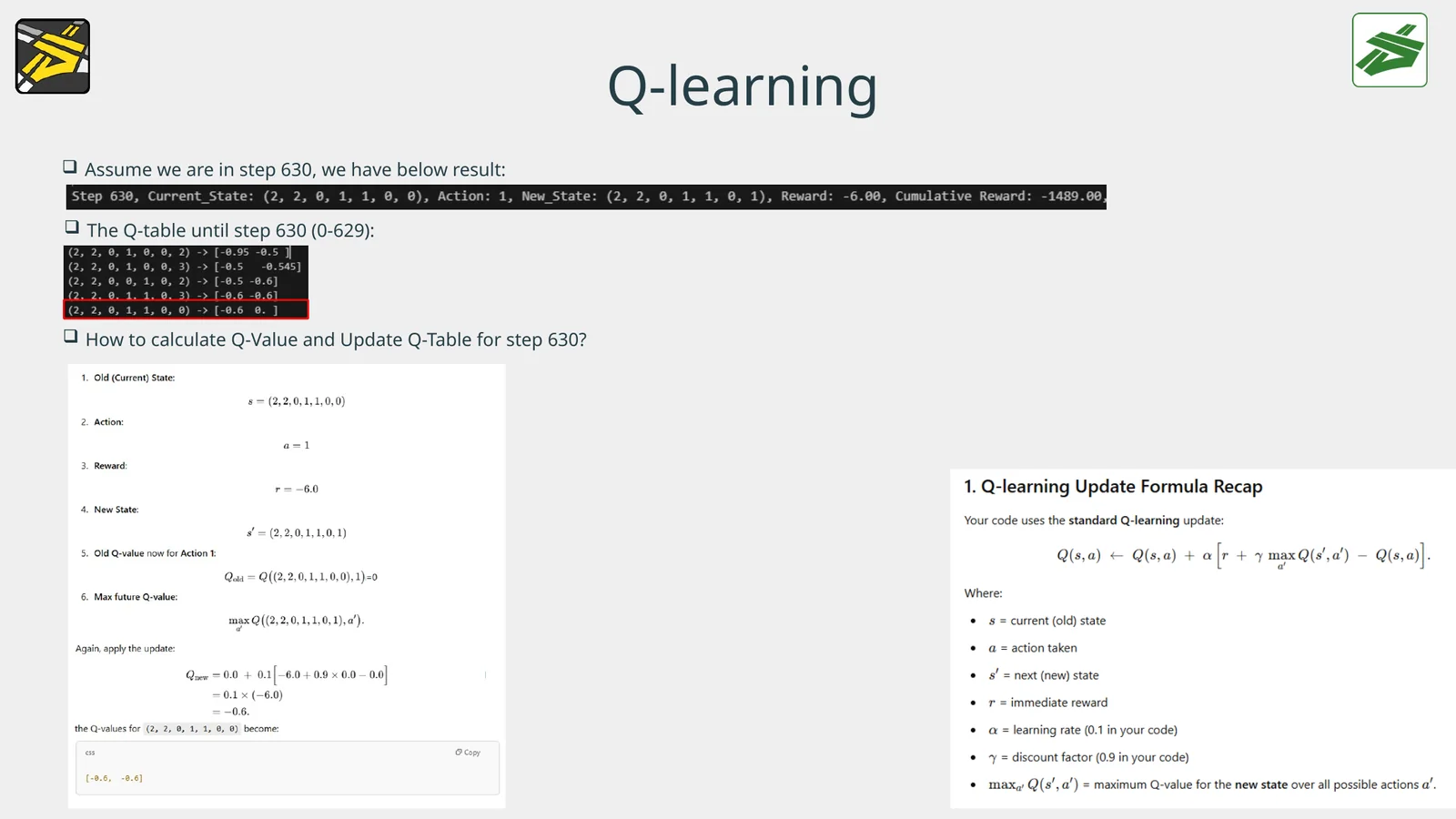
The tutorial frames the control problem as two actions: Action 0 = keep the current phase and Action 1 = switch the phase, subject to the minimum-green-time logic.

Reward

Negative queue length — smaller queues produce a better reward.

Exploration

The agent can explore randomly or act greedily from learned Q-values.

r(t) = −(sum of EB lane queues + sum of SB lane queues)

q_l(t+1) = max(0, q_l(t) + arrivals_l(t) − departures_l(t, phase(t)))

Q(s,a) ← Q(s,a) + α [ r + γ max Q(s′,a′) − Q(s,a) ]

Eight-part Q-learning traffic signal workflow — The tutorial’s Q-learning workflow: reward, state, queue evolution, action, update, exploration, and SUMO variables.

Worked state example

The deck gives a simple example with seven state values:

Current state: (0,0,0,1,0,0,0) → Action: 0 → Next state: (0,0,0,1,0,0,0) → Reward: −1

Worked Q-learning state and Q-value update example — Worked Q-learning example from the tutorial.

Q-learning state action reward and Q-table output — The controller produces state/action/reward information and updates the Q-table/Q-values.

7 • Deep Q-learning

Replace the Q-table with a neural network

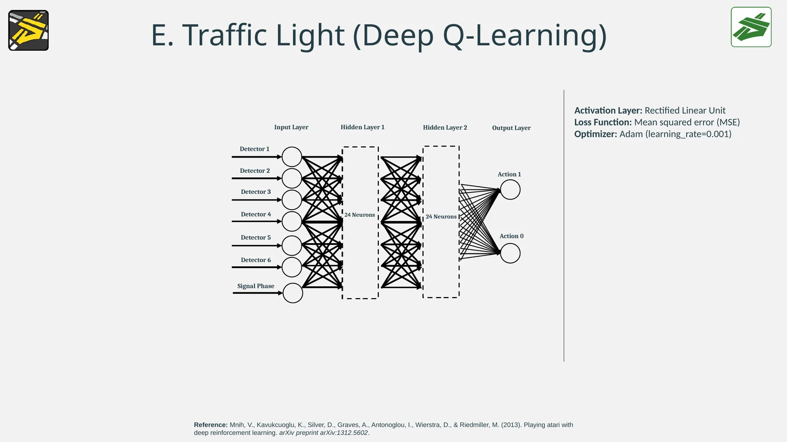
Deep Q-learning keeps the same traffic-control idea but estimates action values with a neural network instead of storing every state–action combination in a table.

Layer	Tutorial configuration
Input	Detector 1–6 + signal phase
Hidden layer 1	24 neurons
Hidden layer 2	24 neurons
Output	Action 0 and Action 1
Activation	Rectified Linear Unit (ReLU)
Loss	Mean squared error (MSE)
Optimizer	Adam, learning rate = 0.001

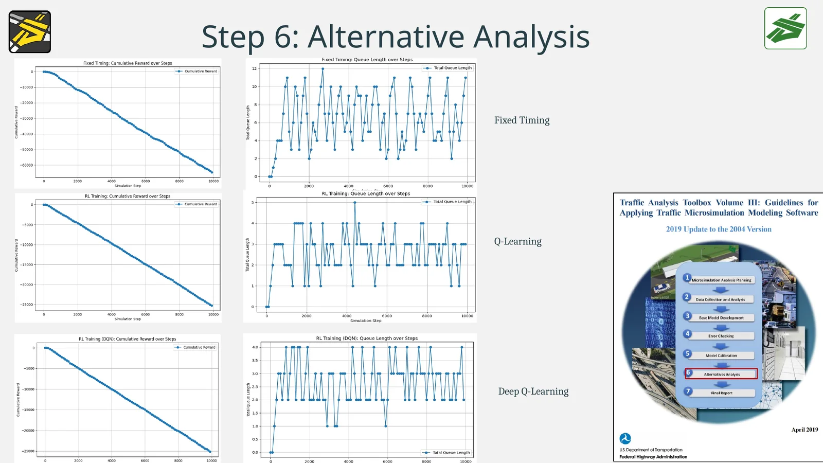
Deep Q-learning neural network with six detectors and phase as inputs — Deep Q-learning architecture used in the tutorial.

8 • Alternative analysis

Compare fixed timing, Q-learning, and Deep Q-learning

The final step compares the three alternatives using cumulative reward and queue-length plots. This is the key evaluation stage: the learning controllers should be judged against the fixed-timing benchmark using the same simulation setup.

Alternative analysis plots comparing fixed timing Q-learning and Deep Q-learning — Alternative analysis plots from the tutorial: cumulative reward and total queue length.

Important: because the example is for tutorial use and calibration is skipped, these plots demonstrate the workflow rather than providing a calibrated real-world performance claim.

Continue with RoadwayVR

Use this page as the conceptual and implementation reference, then follow the RoadwayVR SUMO/Python tutorials to reproduce the traffic-signal experiment and extend it to your own network.

Explore RoadwayVR on YouTube ↗Start with SUMO installation Back to top ↑

Machine & Reinforcement Learning in SUMO

What you will learn